Managing Volatile Tax Collections in State Revenue Forecasts

This report, a joint initiative of The Pew Charitable Trusts and the Nelson A. Rockefeller Institute of Government, will help policymakers better understand how volatile state taxes affect the accuracy of revenue projections. It examines data from 1987 through 2013 and reveals that predicting how much money state governments will raise has become more difficult than ever. The increase in revenue forecast errors is due largely to the growing volatility of tax collections across the states. From 2000 to 2013, the size of fluctuations in tax revenue rose in 42 states. And although no state can entirely eliminate forecasting errors, this study identifies three ways to help them manage volatility.
Overview
During his eight years as the governor of Arkansas, Mike Beebe (D) tried to avoid micromanaging the state government. “With one exception,” he said during an interview for this report. “Money. I’m fiscally conservative. I asked for a report every morning on every aspect of revenue, comparing the daily and monthly collections year over year and comparing those to the forecasts. I did watch those numbers.”1
Beebe had good reason to closely monitor his state’s finances. The amount of money states collect in taxes is harder to predict than ever. And forecasting errors can have serious consequences. Overly optimistic forecasts can prompt hurried, across-the-board spending cuts, tax increases, or borrowing when collections fall short. Alternately, forecasts that are too low can result in a one-time surplus, tempting lawmakers to cut taxes or commit to spending that is unsustainable over the long run.
To better understand how volatile state tax revenue designated for deposit into the general fund affects the accuracy of projections, The Pew Charitable Trusts and the Nelson A. Rockefeller Institute of Government studied errors in forecasting state revenue by examining personal income, sales, and corporate income tax data from 1987 through 2013.2 The analysis updates a 2011 study and includes findings from a new survey of state officials.3 It also draws from current literature and interviews with government finance experts and elected officials. The research shows that:
- Forecasting errors are on the rise, and the increase is driven by the growth of revenue volatility—year-to-year swings in tax collections.
- Corporate income taxes are the hardest to estimate; sales taxes are relatively easier.
- Estimating errors are larger during and after recessions but also occur during expansions.
- Smaller states and those that are dependent on a limited number of economic sectors for their tax revenue tend to have larger percentage errors than more populous or economically diverse states.
- The timing of forecasts matters; the longer the time between the forecast and adoption of the state budget, the less accurate estimates will be.
- Changing the mix of taxes in a state does not necessarily improve the accuracy of revenue forecasts.
No state can entirely eliminate forecasting errors. Unexpected economic turns, new legislation, the rise and fall in housing values, and changes in federal policy, such as the 2013 budget deficit reduction plan known as the “fiscal cliff,” guarantee that estimating revenue will always be imprecise. These factors can drive revenue volatility, contributing to the difficulty of accurately estimating the money coming into state coffers. And the resulting shortfalls or surpluses may complicate lawmakers’ efforts to craft and execute balanced budgets over several years.
Pew’s research demonstrates that an effective way to manage unpredictable revenue is by designing an evidence- based reserve, or rainy day, fund that is built upon an understanding of economic changes that affect revenue. The ideal fund would include a provision tying reserve deposits to unexpected windfalls and have a maximum size based on observed patterns of volatility in the state.
In addition, Pew recommends that state officials prepare and update revenue estimates as close as possible to the start of the budget year and that they regularly analyze errors and sharpen forecasting techniques and assumptions to reflect changing economic conditions.

Fiscal 50: State Trends and Analysis
Limits of the Study
Though our research determined the percentage size of individual states’ forecasting errors over the 27 years, we caution against comparing or singling out states. For one thing, nine states do not tax personal income, and we are missing three years of data for one of those states, Texas. Large errors do not mean a state’s forecast methods are flawed. Natural disasters or unexpected economic events can throw forecasts off track at any time, as was observed during the Great Recession of 2007 to 2009 and the relatively slow recovery that has followed.
Increase in forecasting errors is driven by growth of revenue volatility
Over the 27-year period covered in this study, forecasting errors have gotten larger because revenue has become increasingly volatile. This is especially true for the three recessions and three economic expansions that took place during the study period. The forecasting errors of the last two recessions (2001 and 2007) were larger than those of the previous one in 1990. The greater the error, the more difficult the budget challenge. In 2009, the worst year of the Great Recession, more than half of the states expected tax collections to be higher than they actually were.
The size of estimating errors has grown larger in part because revenue is increasingly more volatile. In fact, volatility increased in 42 states between 2000 and 2013, according to a recent analysis by the Rockefeller Institute of Government.4 The increase in errors has not occurred because forecasters are any less adept than in the past. If anything, the science of estimating tax collections has improved markedly due to advances in information technology.
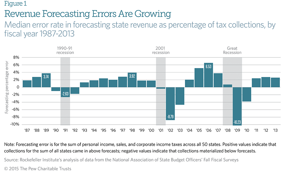
From 1987 through 2013, there were three periods in which state revenue forecasts were sharply negative or when officials overestimated tax collections and states had to close budget gaps. Each corresponded with either the 1990-91, 2001, or 2007-09 recessions. The errors in the latter two recessions were more than three times as large as the error in the earliest.
A common measure of volatility over time—standard deviation—also demonstrates how hard it has become to accurately predict revenue. The standard deviation of the year-over-year change in total tax revenue for all 50 states was below 3.5 percentage points every year between 1987 and 2001, after which it began rising to exceed 6 percentage points from 2009 through 2011. A low value means that the change in revenue is similar from year to year. The higher the value, the more dramatic the revenue fluctuation.
World Economy Is Altering State Revenue Forecasts
Conditions in countries outside the U.S. are influencing revenue forecasts in many states, according to budget officials.
The value of the yen is important in Hawaii, where Japanese tourists are a key market. Michigan monitors the strength of the Chinese economy; General Motors sells more cars in China than it does in the U.S.* The Pacific Rim economy is vital to Nevada, where sales and gaming revenue are affected by high-rolling baccarat players from Asia. “[The] Chinese New Year goes into my [forecasting] model and that’s impacted by the health of the Asian economy,” says Janet Rogers, chief state economist.†
Political unrest in the Middle East could affect oil supplies and prices and, in turn, revenue in Oklahoma and other energy states. Maine’s largest corporate taxpayers have shifted from smaller domestic companies to nationwide or even worldwide retailers. “Today, you’ve got to be aware of what’s going on in the nation, the region, and the world, not just what’s going on down the street,” says Michael Allen, chairman of the Maine Revenue Forecasting Committee.‡
* “General Motors Sets Sales Record in China,” news release, General Motors, Dec. 3, 2014. http://media.gm.com/media/us/en/gm/news.detail.html/content/Pages/news /cn/en/2014/Dec/1203_sales.html.
† Janet Rogers (chief economist, state of Nevada), interview with The Pew Charitable Trusts, June 2014.
‡ Michael Allen (chairman, Maine Revenue Forecasting Committee), interview with The Pew Charitable Trusts, May 2014.
Corporate income taxes are the hardest to estimate
Nowhere is volatility greater than with corporate income tax revenue. The data showed that the median forecasting error rate over the 27 years was 2.8 percent for the corporate income tax compared with 1.8 percent for the personal income tax and 0.3 percent for the sales tax. Of the three, corporate taxes make up the smallest share of state revenue; personal income taxes make up the largest.
State forecasters, mindful of the historic volatility of corporate profits, take a cautious approach to forecasting this revenue. The reason is simple, says Barry Boardman, North Carolina’s chief economist for the General Assembly: “It’s easier to manage a surplus than a shortfall.”5 Looking across any five years of North Carolina data, Boardman says, corporate taxes usually swing up or down 30 percent. With that much volatility, he says, it is better to be conservative in estimates even when profits are going up. The downside of underestimates, however, is that lawmakers are limited in the amount of revenue they can spend. “But history tells us that while we may be overly cautious, that caution plays well when things turn the other way and doesn’t leave them in a position where they have overpromised,” Boardman says.
Even when forecasters are cautious in predicting the amount of corporate taxes that a state will collect, revenue volatility can surprise. Near the end of fiscal year 2014, several states with conservative estimates were caught off guard by declines in corporate tax revenue. Delaware was suddenly confronted with a budget gap because corporate income taxes came in $70 million below estimates.6 Tennessee and Oklahoma had the same problem. Louisiana officials have been confounded in their estimates by a precipitous fall in corporate income and franchise tax collections, from $1 billion a year in 2008 to $335 million in 2013. “If that comes back up much, it will surprise us,” says Jim Richardson, a Louisiana State University economist and member of the panel that estimates revenue. The puzzle is that Louisiana’s corporate tax base is largely made up of petrochemicals and oil and gas, which weathered the recession relatively well. The number of tax credits doled out to energy companies has risen, but that does not completely explain the drop either, Richardson says.7
Capital gains throw off estimates
While the unpredictability of corporate taxes is well known, many state officials say they have been surprised in recent years at the increase in volatility of sales and personal income tax collections. For personal income taxes, the most volatile component is capital gains, which are largely contingent on an unpredictable stock market as well as other factors, such as investor behavior, that are difficult to anticipate. For example, stock prices may go up, but individuals may choose not to sell their holdings. Or the market may be flat, but because of prospective changes in tax law, people realize capital gains that have accumulated over a number of years. Additionally, a significant portion of capital gains comes from the sale of businesses, and during recessions or economic slowdowns, that activity dries up.
The magnitude of capital gains-related volatility tends to be large relative to state budgets. The 10 states that depend the most on capital gains revenue are, in descending order, New York, California, Vermont, Connecticut, Oregon, Hawaii, Massachusetts, New Jersey, Idaho, and Colorado.8
California, with its progressive personal income tax structure that applies higher rates to wealthier individuals, offers a good example of this kind of volatility. The state taxes capital gains at the same rate as other income so when stock prices go up, as they did in 2013, revenue also increases because of high-income taxpayers who sell equities.
The reverse is true when stock prices fall. In 2007, before the recession hit, capital gains contributed about $11 billion, or 9 percent, to California’s general fund. In 2009, capital gains revenue dropped to $2 billion, or 3.5 percent of the general fund. The 2014-15 budget relies on almost 10 percent of revenue coming from capital gains.9 These wide fluctuations perplex forecasters and increase the size of estimating errors, compared with states that depend less heavily on capital gains. California’s reliance on capital gains revenue for its general fund and on taxes paid by a small, wealthy portion of its population led Governor Jerry Brown to propose tying the state’s rainy day fund to volatile capital gains revenue, which California voters approved Nov. 4, 2014, through a ballot initiative.10
The wide variation among states that estimated capital gains in 2013 illustrates the imprecision in modeling revenue. Initial forecast estimates of year-over-year decline in capital gains were 8.3 percent in Arizona, 44 percent in California, 31 percent in Massachusetts, and 2.6 percent in New York. All later revised those estimates; for example, Massachusetts officials said the 31 percent decline would be followed by a 22 percent increase in 2014 and then only a 6 percent increase in 2015, demonstrating the unpredictable nature of capital gains.11
One of the trickiest issues surrounding capital gains is that the timing of tax collections associated with this type of income depends on the economy and taxpayers’ behavior. The spike in collections during the recent federal budget showdown called the fiscal cliff exemplifies how taxpayers’ actions can add to volatility. Throughout 2012, many high-income taxpayers realized that their rates could go up in January 2013, because Congress was signaling it would not renew tax cuts enacted during George W. Bush’s presidency that were scheduled to expire. In response, many taxpayers accelerated capital gains into 2012 to take advantage of the lower rates. Such changes also affected state income tax revenue, and forecasters could not predict by how much taxpayers would shift capital gains realizations from 2013 to 2012. The resulting 2012 surge in capital gains was basic tax planning for payers and led to unusually high collections when taxpayers filed their 2012 tax returns. For 2013, capital gains filings were much lower.
Although forecasters were not caught entirely off guard by this drop in revenue, they were surprised by the size of the shift. On the state level, this resulted in increased revenue in fiscal 2013, which included the last half of tax year 2012, and then in revenue shortfalls in fiscal 2014. Because many states underestimated the impact of this one-time event, they experienced painful budget gaps, which compounded the challenge for forecasters in states that reduced income tax rates, among them Kansas, Maine, Michigan, Nebraska, North Dakota, and Ohio.
Usually reliable sales tax collections baffle forecasters
For some states, the sluggish recovery from the Great Recession has led to weaker-than-usual growth in sales tax revenue that has amplified forecasting errors. Sales tax collections usually are the easiest revenue source to estimate because purchases of such things as food and toiletries typically hold steady regardless of the economy’s performance. But consumers dramatically curtailed spending even on staples during the recession, causing the sharpest drop in sales tax receipts in 50 years. Even after consumers resumed more normal buying habits, sales tax collections have been growing so slowly that in many states they are still below prerecession levels.12
Furthermore, sales tax revenue can be destabilized when it is contingent on certain big-ticket items whose sales suffer during a recession. For example, as much as 40 percent of Maine’s sales tax base at times can come from purchases of motor vehicles, boats, and building supplies, a narrow set of sources that can usually withstand downturns. But in a housing-led recession such as the last one, “the bottom just fell out,” says Michael Allen, chairman of the Maine Revenue Forecasting Committee. “The two areas that were hurt the hardest were residential homes and auto sales. At times it can be extremely volatile.”13
Kentucky’s recurring budget shortfalls occur, in large part, because its revenue is growing more slowly than its economy. Sales tax receipts, which make up a third of the state’s general fund revenue, declined only once between 1979 and 2007 but have fallen three times in the past five years, according to Greg Harkenrider, chief state economist.14 Part of the reason for the drop, he says, is that the elasticity of the sales tax has decreased. Elasticity is a measure of how much tax collections go up or down in response to economic changes. A high value means that the tax responds dramatically to changes in economic conditions, and a lower value means it reacts less significantly. When determining the state’s revenue estimates, Harkenrider says, officials used to routinely assume growth in sales tax collections of between 5 and 7 percent a year. “Now, 3 percent is the new ‘good,’” he says. “It’s very clear the elasticity of the sales tax has gone down.” In addition to the fact that consumers and businesses have been more guarded in spending, the way they purchase goods and services (e.g., online purchases or direct purchases of digital content) has changed and may not be taxed. Furthermore, the sales tax base in many states is relatively narrow, often excluding groceries, drugs, motor vehicles, gasoline, online purchases, and most services. Despite efforts to update state tax laws to keep up with evolving consumption habits or to expand the base, many state sales tax policies do not reflect current conditions. In Kentucky, Harkenrider relates, state officials are exploring whether to expand the sales tax base because consumption- based tax collections have fallen.
How States Estimate Revenue
A combination of science and art, the revenue estimating process usually begins with national and state- specific economic forecasts developed by economists inside and outside the state. These reports include data, such as predicted population changes, wages, employment, personal income, interest, consumer confidence levels, gross national product, and stock market performance, as well as assessments of important sectors in the state, including automobile production in Michigan or tourist visits and spending in Hawaii.
These data are fed into computer models that forecast the amount of tax revenue the state could generate. The models include historical revenue trends for similar economic conditions, tax returns likely to be filed in the forecast year, tax increases and policy changes approved in the past year, and surveys of consumer confidence in the economy that could predict spending patterns. States even have models for revenue loss from past natural disasters that they use to estimate the impact on tax collections of any recent calamities. Pew’s research is consistent with other studies concluding that the methods states use to forecast tax collections are not significantly correlated with the size of errors.
In most states, according to our survey of state officials, the executive branch’s revenue office and legislative staff both prepare revenue forecasts, often offering officials a choice between optimistic, pessimistic, and in-between numbers. In seven states, the governor’s office alone prepares the estimates.* In four, an independent group of academics, business leaders, and elected officials appointed by the governor and lawmakers determine the estimates.† Whatever the structure, participants review the data and come to an agreement on a single number in more than two-thirds of the states.
* The seven states are Arkansas, Georgia, Minnesota, New Jersey, Oklahoma, South Carolina, and West Virginia.
† The four states are Hawaii, Nebraska, Nevada, and Washington.
States with small populations make larger errors
Frequently, the smaller the state’s population, the larger the forecasting error.15 This may reflect the fact that smaller state economies often are less diverse than those in more populous states and may be more easily dominated by one or a few industries that can cause significant year-to-year swings in revenue.
Idaho, which ranks 39th in population, has consistently underestimated both its rate of economic growth and its tax collections.16 Chief Economist Derek Santos, who prepares the initial estimates for the governor and Legislature, attributes the errors to volatile corporate income taxes, a circumstance in which large employers can have an outsize impact on collections. Idaho’s largest corporate taxpayer is Micron Technology, which contributed to the state’s volatility and revenue estimation difficulties when its corporate revenue did not grow as planned during the Great Recession, leading to cuts in overhead costs that included layoffs.17 This occurrence happens in other small and large states where revenue forecasters use and are reluctant to challenge companies’ estimates for the number of workers they employ. Washington state forecasters, for instance, historically have accepted Boeing’s productivity and workforce assumptions only to see the company fall short of those goals.
States that rely on a few sectors of the economy have larger errors
North Dakota is both small—ranking 48th in population—and dominated by a few industries. The data show that it had the largest forecasting errors of any state, mostly because of its transformation during the 2000s from a primarily agricultural economy to one centered on energy production.18 Forecasters simply have not been able o predict the fast growth of the oil and gas industry, which poured people and revenue into North Dakota even during the Great Recession when most states were struggling. The forecasting errors—as high as 69 percent— have resulted in budget surpluses. In the two-year budget cycle ending June 30, 2013, general fund revenue was about 48 percent, or more than $1.6 billion, above the forecast.19 “It’s a problem on the good side that continues to surprise us,” says Governor Jack Dalrymple, who previously served as House Appropriations Committee chairman in the state Legislature.20
Until the completion of the first shale oil wells in western North Dakota in 2006, officials estimating tax collections mostly worried about the impact of farm commodity prices. With the oil boom, everything changed, says Pam Sharp, the state’s revenue director.21 Officials had to predict revenue not only from mercurial energy severance taxes but also from sales taxes on oil rig equipment. Sales and income tax collections skyrocketed as employment rose 26 percent—the highest in the nation—between 2007 and 2013.22 The growth in gross domestic product was more than five times the national average.23 “The industry ramped up so quickly,” Sharp says, explaining the revenue twists.
Because mineral prices are inherently volatile, so are energy revenue estimates.
But even surpluses have drawbacks. Elected officials struggle to manage the competing budgetary priorities that accompany growth, such as the size of tax cuts, reserve funds, and heightened demands on infrastructure. As a legislator, “You don’t have a good sense of how much is enough,” says Thomas Fiebiger, a former North Dakota state senator.24 State officials asked Moody’s Analytics, which prepares the state’s economic forecasts, to revise its model to reflect the rapid expansion of the oil industry in time for the 2013-15 budget cycle. Nevertheless, through February 2014, general fund revenue was about 6 percent above the forecast made in May 2013.25
Though North Dakota’s growth is an anomaly nationwide, the state’s tendency to underestimate revenue is not. The officials Pew interviewed there said that while they attempt to be as accurate as possible, given a choice they would rather err on the side of underestimating revenue, especially after the big misses during the Great Recession, than overestimating and winding up with a budget shortfall.
In Wyoming, natural gas, coal, and oil drive the economy; taxes generated by gas production are the state’s single biggest revenue source.26 Because mineral prices are inherently volatile, so are revenue estimates. Governor Matt Mead still seethes about an unexpected 75-cent drop in natural gas prices in January 2012 that lowered revenue projections by $100 million a month after he had proposed a balanced, two-year $3 billion spending plan. Gov. Mead cut the budget to close the shortfall. Since then, he says, gas prices have gone up and the forecasts, made with the advice of mineral companies, have been “surprisingly accurate. They are very conservative in their estimates because we don’t want to be left in the lurch.”27
Both Hawaii’s and Nevada’s main source of revenue is tourism. All its aspects—visitor arrivals and spending, hotel room rates, airfares, and exchange rates, particularly for the Japanese yen—have a bearing on Hawaii’s revenue. Revisions in the state’s revenue forecasts for fiscal 2014 tell the story. As 2013 began, the Council on Revenues, which makes the projections, cited the strength of the tourism sector in raising its estimate of year- over-year growth in tax collections three times, to a high of 8 percent, for fiscal 2014. But then, toward the end of 2013 and beginning of 2014, the council lowered its forecast three times as it became clear that tourists were
spending less money.28 Instead of assuming revenue growth at 8 percent, the panel concluded that zero growth in revenue would occur between fiscal 2013 and 2014.29
The abrupt change created an instant $180 million budget gap, and officials covered it with reserves.30 The downward forecasts also led to shortfalls in the 2015 and 2016 budget years, which lawmakers will have to address. “Being tourism-dependent means that we focus more on tourism in our assessment of the tax picture, and that we are more influenced by global events than some [state] economies are,” says Carl Bonham, a member of the revenue council and executive director of the University of Hawaii’s Economic Research Organization.31
Nevada also has to watch for changes in tourist behavior and competition from other states that affect revenue estimates. Though this report does not look at gaming revenue, those collections have a ripple effect on sales taxes. In the past few years, state officials say, visitors to Nevada have been spending less on gaming and more on nongaming activities, including nightclubs, shows, and shopping. “Our visitor volume is at historic highs, but they’re not coming just to play the slot machines,” says Janet Rogers, chief state economist.32 The take from the tax on casinos proves Rogers’ point: Nevada now brings in about $687 million a year from gaming, down from $1 billion.33
Timing of forecasts can affect accuracy
Our survey of state officials shows wide variation in when states prepare forecasts for the coming budget year,34 but certain practices are common among most states. For example, many release their forecasts toward the end of the calendar year to inform a governor’s budget proposal before January. A second forecast typically comes during the spring or early summer in case the governor and lawmakers need to make adjustments before the fiscal year begins July 1. Most states also take a long-term approach to estimating revenue and offer forecasts of tax collections for two or more years. Alaska even looks nine years ahead because of the volatility inherent in its dependence on energy revenue. But while these general outlines are typical, differences exist in the timing of forecasts prepared for the governor and Legislature to develop the budget.
Alabama, for instance, prepares its estimates as early as eight months before the start of the July 1 fiscal year. On the other hand, Delaware, Pennsylvania, and Tennessee complete their final forecasts about two weeks before the budget year begins.
States on a two-year budget cycle update their second-year forecast to account for tax adjustments approved by the Legislature and changing economic conditions. Because the lag between preparing the initial forecast and the one used in the adopted budget is longer in the second year of a biennium, these states usually make greater estimating errors. The data show that the accuracy of a revenue estimate worsens by more than a percentage point for the second year of a biennium and by about a half of a percentage point for every 10 weeks of lag between the time a forecast is prepared and the start of the forecast period. These phenomena can be eased by states adjusting their estimates carefully during a biennium’s second year.
States are not likely to meaningfully improve their revenue forecasts by streamlining their tax structures; it is critical that officials put policies in place to manage volatile revenue. The most consistent, flexible solution is an adequate rainy day fund.
Changes in tax law complicate revenue estimates
Some states have restructured their mix of taxes to broaden the base and reduce volatility. Ohio began replacing its corporate income tax in 2006, shifting to a commercial activity tax that officials say is less volatile.35 Rhode Island changed its income tax rate and expanded its sales tax base to include previously exempt goods and services.36 North Carolina shifted from a more progressive income tax to a flat rate, while also creating a simpler system by eliminating a number of deductions and tax credits. Michigan scrapped a business tax that was notoriously hard to forecast because it included 40 credits dependent on many difficult-to-gauge factors.37
While such tax changes may help control revenue volatility, they complicate the revenue forecasting process in the short run. With any new tax, it takes several years to compile enough data on receipts to understand the factors affecting revenue strength or weakness. Until forecasters have those observations in hand, they may have little evidence to use in fine-tuning their estimates of how much revenue tax law changes will raise or cost.
In Ohio’s case, the dramatic economic shifts that occurred as the commercial activities tax was being phased in added complexity, with revenue initially underestimated before the Great Recession and then overestimated as the economy declined. Ross Miller, chief economist for the state’s Legislative Service Commission, said it is probably going to take a few more years to understand all the economic variables that affect the flow of revenue.38
Michigan officials say they believe that revenue from the state’s new corporate income tax eventually will be easier to predict than the two business taxes it replaced, one of which included some still-active tax breaks that continue to affect revenue estimates.
In North Carolina and elsewhere, determining whether shifts in tax collections are due to the tax changes in 2014 or the state’s overall economic performance is complicating the job of predicting revenue. “I’m going to feel much better about a forecast in 2016 because I’ll have [two years of] the tax law changes under my belt,” says North Carolina’s Boardman.39 Initial estimates made in July 2014 by the legislative fiscal research staff showed that income tax collections would be $880 million lower than forecast over the next five years.40
Moreover, tax policy changes that are specific to narrow elements of a state’s economy can prove just as disruptive to the accuracy of forecasts. The 2009 expansion of Oregon’s business energy tax credit provides a good example of the hazards of trying to estimate a tax change. Instead of up to $40 million projected growth in credits over two years, the state found itself on the hook for an additional $200 million in credits. Officials responded by capping the credit.
Pew recommends that states regularly analyze errors and sharpen forecasting techniques and assumptions to reflect changing economic conditions.
Recommendations
States would have to make drastic changes to their tax structures in order to substantially reduce revenue volatility—changes that would be apt to come with trade-offs between competing tax policy priorities and significant costs. As such, states are not likely to meaningfully improve their revenue forecasts by streamlining their tax structures; it is critical that officials put policies in place to manage volatile revenue.41 The most consistent, flexible solution is an adequate rainy day fund.
Build budget reserves and design them to harness volatility
Reserves act as a buffer against unexpected shocks by replacing lost revenue from predicted shortfalls triggered by downturns, natural disasters, the rise and fall of commodity prices, and other factors. In this way, states can curtail cuts in services and tax increases. Healthy reserves also can help keep borrowing costs down because credit rating agencies view them favorably when rating state debt.
Regularly setting aside money in reserves often requires balancing short- term gains with a long-term view of fiscal health. Dollars deposited into rainy day funds cannot be spent on programs, tax cuts, or debt service but can help offset revenue losses in future downturns. Nearly every state lacked enough in reserves to mitigate the severe revenue declines incurred during the 2007-09 recession. Based on that experience, many state officials say they hope lawmakers will set aside more money in budget stabilization funds going forward.
Georgia, Nevada, Oklahoma, South Carolina, Tennessee, Vermont, and Virginia have raised the cap on the size of their rainy day funds after the recession.42 Further, states that have had relatively large forecasting errors, including Kentucky, Maine, Mississippi, North Carolina, and Oregon, do not have equally large amounts of money set aside in reserves to help counter the effects of volatile revenue.
“One of the things we learned was that the levels of reserves that we thought were appropriate prior to the recession may not have been healthy enough,” says George Naughton, chief financial officer in Oregon, which set up its rainy day fund just before the recession hit in 2007.43 The state has prudently charted a path to increase its two reserve funds from 0.5 percent of general fund revenue at the end of the 2011-13 biennium to 2.5 percent by the end of 2015 to 9.6 percent by the end of 2021. The cap on the combined funds is 10 percent.
Connecticut drained its $1.4 billion rainy day fund during the worst days of the recession in 2009, borrowed $1 billion for operating expenses, and deferred $50 million in required public pension payments.44 Governor Dannel Malloy, who says he came into office determined to rebuild reserves, convinced lawmakers to deposit the entire fiscal 2014 budget surplus into the rainy day fund, boosting it to $392 million.45 “No government should have exhausted its rainy day fund,” he said. When asked if this applies even during a severe recession, he replied, “Who’s to say tomorrow won’t be even tougher?”46
Other states have had a particularly difficult time restoring reserves to desired levels. Nevada, which was hit especially hard by the last recession, has struggled to rebuild its depleted stabilization fund. Lawmakers there and elsewhere say they first needed to funnel additional revenue to programs cut during the recession, such as education, before bolstering reserves. Fred Church, Ohio’s deputy budget director, says debates about maintaining and increasing reserves often encounter resistance, including the political obstacle of convincing elected officials to pile up savings. “Once you’ve accumulated large reserves, there’s pressure to spend it or give it back in tax cuts or rebates.”47
To help lessen that pressure, Pew recommends that states establish rules tying rainy day fund deposits in part to overall revenue volatility or a single unpredictable tax so that some of the revenue stemming from unusually good times is automatically deposited into reserves instead of spent on other priorities. Thirteen states have enacted such rules:
- Hawaii, Idaho, Tennessee, Virginia, and Washington connect rainy day fund deposits to overall fluctuations within their major or total revenue streams. Virginia set up a consistent policy to save during years when revenue is growing. It is based on a formula comparing how the state’s major taxes performed in the most recent budget year with the average revenue growth over the preceding six years, or the trend growth rate. Half of the money above the trend rate is automatically socked away in the stabilization fund.48
- Alaska, California, Louisiana, Massachusetts, and Texas tie deposits to specific volatile taxes. In Alaska, Louisiana, and Texas, officials target oil and natural gas revenue. Texas brings in a large part of its stabilization fund from growth in severance taxes on oil and gas production. Three-fourths of severance tax revenue above the benchmark year of 1987 is put into the fund, which swelled to $8 billion in 2013 and is growing along with the industry. Despite this success, Texas’ fund structure poses some challenges. Basing deposits on oil and gas revenue from 25 years ago may be incompatible with current conditions. Massachusetts’ deposit rule requires the state to put capital gains revenue above a threshold that grows with the economy—$1.05 billion for fiscal 2015—into reserves. In California, which also has volatile capital gains revenue, voters approved a ballot measure in November 2014 to allow state officials to structure the reserve so it captures excess capital gains tax collections during boom years and a fixed 1.5 percent of California’s general fund each year.
- Arizona, Indiana, and Michigan base deposits to the rainy day fund on fluctuations in personal income, which reflects overall economic conditions instead of ups and downs in specific revenue sources. This approach works particularly well when the economy is strong and officials can set aside money for tighter times. However, this approach does not work as well in states where revenues and the overall economy do not move closely in tandem.
Before designing rules for rainy day funds, state officials should analyze fluctuations in revenue through regular studies. Utah is an example of a state that uses regular revenue studies to inform policy decisions. Lawmakers there approved a plan in 2008 to study revenue volatility every three years, focusing on the factors and trends influencing it. As a result of these studies, legislators have twice increased the limits on the state’s two budget reserve funds.
Cut the lag between the revenue forecast and the start of the fiscal year
This research has shown that state officials benefit from preparing and updating revenue estimates as close as possible to the start of the budget year. Many states follow this practice, which is sensible because it gives officials more timely information about spring income tax collections. It does not provide a complete picture of such collections, however, because it covers only returns filed by the April deadline. Extensions, which are typically filed by upper-income individuals, also can produce surprises.
For years, Maine estimators had prepared a forecast for the biennium on Dec. 1, with a revision on March 1. Then in mid-March, corporate filers made their final income tax payments for the previous calendar year, and on April 15 many individuals paid their income taxes. “You could be blown out of the water,” says Allen of the Maine Revenue Forecasting Committee.49 “We’d put out this new forecast on March 1 and [the legislators] would react to it and two months later, in some years, you’d have a big April surprise and be awash in revenue. Or it would go the other way and you’d have to start all over again. It just didn’t make any sense.” As a result, lawmakers changed the date of the revised forecast to May 1, giving them better information closer to the start of the budget year.
Analyze errors, tweak assumptions, and ask for help
State revenue estimators should regularly examine their methods and errors. This undertaking applies not only to the economic models used but also to the revenue models, which often receive less attention.
Many forecasters already test their work by trying out alternative scenarios, which today’s computer technology can run in minutes instead of hours as in the past. Similarly, forecasters are always comparing actual revenue with what was forecast. “We know that we will be asked by the governor or key legislators, or the press, so we want to be prepared with the facts and the reasons why we are off,” said Thomas Stinson, chief economist for Minnesota for 26 years before his retirement in 2013.50
Kentucky’s Harkenrider, who has helped forecast the state’s revenue since 1996, says he advises officials to use more than one analytical model and combine the results. “I’m an unapologetic blender,” he says. “I run six or seven different models, look at the answers and blend those.” Patterns of tax collections change, he says, so estimators need to have an intimate knowledge of their states’ data to make adjustments from year to year. “On sales tax, for example, if I use only data from the 1980s and 1990s, I will get a higher estimate than if I use data from the last 10 years,” when sales taxes were more volatile, Harkenrider says.51
Hawaii is evaluating its State Council on Revenues’ forecast history. Bonham, the University of Hawaii economist, says he has argued for estimates with confidence intervals that measure the reliability of an estimate. “At a minimum we could include with our submitted consensus forecast a range that reflects the disagreement of the council,” he says.52
Reasonable economic assumptions often change, and forecasters should factor those modifications into their estimates. For years, the conventional wisdom about Nevada was that state revenue would not fall sharply during recessions because tourists would still come to gamble. This held true in 2001 when the recession produced a relatively minor dip compared with other states. But during the Great Recession, a fall in tourism coupled with the housing crisis caused Nevada’s revenue to plummet more than most states. Today, Nevada faces a new threat to revenue from increased gambling competition in other states. Chief State Economist Janet Rogers says there is a downside to relying too much on historical knowledge. Estimators had a harder time forecasting tax collections in the most recent recession, she says, “because we had not experienced this kind of pullback historically.”
Some states have added outside experts to assist state estimators, mostly with regard to the broad parameters of the economy. After a series of inaccurate revenue forecasts, especially for corporate income taxes, Oklahoma is moving to contract with independent experts, including economists and oil and gas industry analysts. The state already uses Oklahoma State University professors for its economic assumptions. The idea is to agree upon a consensus forecast to present to state officials.53
Consensus Revenue Forecasts
No revenue study, including this one, has proved that consensus forecasting increases accuracy or improves the forecast itself. Nevertheless, arriving at agreement among the governor, lawmakers, and other parties on a single estimate is beneficial for obtaining acceptance of the forecast. State officials concur; about two- thirds of the states have adopted a consensus forecasting system. In most of these states, the law requires the governor and Legislature to use a consensus figure in preparing the budget.
The participants in the consensus process vary. In most states, a formal group of economists, executive and legislative branch officials, lawmakers, and sometimes residents hold public meetings to bring together competing forecasts and decide on one or a blended result. Indiana’s consensus panel even attempts to reach an agreement on the methodology that produces the predicted revenue number.* In Connecticut, the consensus group meets in November, January, and April. The January estimate is required for the governor’s budget proposal, and the Legislature is compelled to use the April forecast for its adopted budget. North Carolina’s consensus group is more informal; neither the governor nor Legislature is required by statute to use the consensus estimate.
The trend toward the consensus approach has accelerated in the past 20 years as state officials sought to reduce the political infighting that often accompanies forecasts. Iowa used to allow the governor to determine the revenue number, and lawmakers would argue about it for much of the legislative session before choosing their own estimate. “Before, it used to be dueling estimates,” says Iowa Governor Terry Branstad, speaking of a time around two decades ago. “Now, we have one number and everyone works off of it.”† Maine went through a similar experience, with lawmakers sleeping one night on cots in the statehouse to meet a budget deadline that had been missed because of accusations of political manipulation of revenue estimates. The independent consensus process now in place eased that tension, says Maine’s Michael Allen.
“We’ve had consensus forecasting in place since 1987,” says Louisiana State University’s Jim Richardson. “Does it forecast correctly all the time? No. But in our case, it says that forecasts are not driven by politics. They are driven by financial and economic factors.”‡
John Mikesell, a professor at Indiana University and a member of that state’s consensus revenue forecasting panel, says too much emphasis on depoliticizing the process may miss the inevitable realities of budgeting. The forecast should be as accurate as possible, he says, but it also needs to be regarded as binding by those building and executing the budget. Indiana’s process is designed to explicitly recognize politics, he argues, because the forecasting panel always includes Republicans and Democrats, reducing political pressures to put forth artificially high or low results. The goal then becomes to produce a reasonably accurate, unbiased estimate and, because all political views are included, to have that forecast regarded as the revenue ceiling in all aspects of the budget process.”§
In some states, a sole entity estimates revenue. New Jersey’s forecast is done by the governor’s office, with no formal process in place. The estimates have been a constant source of friction between Republican Governor Chris Christie and the Democrat-controlled Legislature. The Legislature’s budget officer has produced lower revenue estimates than those of the governor’s chief economist, prompting Christie to dub him “Dr. Kevorkian of the numbers” and to call for his dismissal.|| Most recently, Christie’s own chief economist resigned this year following three straight years of estimating errors.#
Similar disputes have occurred in the past in Montana, where the Legislature develops that state’s official forecast. Former Governor Brian Schweitzer had consistently challenged the numbers. New Hampshire also has a history of sparring between the governor and lawmakers. Governor Maggie Hassan created a consensus-estimating panel in 2013 but did not include lawmakers as formal members of it. As a result, the Legislature has said it would do its own estimates.**
Ohio officials defend their system in which the Legislature chooses the revenue estimate for the budget with some consultation with the governor’s office. “There’s no formal consensus, which is not to say that we don’t talk, share information, and move towards each other, which we do,” says deputy budget director Church. “This is one of the things that nettles me, honestly, about the rating agencies and some of the independent groups that seem to feel that if you don’t have some sort of binding consensus, it implies that each group does what it does in a vacuum. That is not the case.”††
* John Mikesell (professor, School of Public and Environmental Affairs, Indiana University), email correspondence with The Pew Charitable Trusts, July 2014; John L. Mikesell and Justin Ross, “State Revenue Forecasts and Political Acceptance: The Value of Consensus Forecasting in the Budget Process,” Public Administration Review 74, no. 2 (2014): 188–203, doi:10.1111/puar.12166.
† Terry Branstad (governor of Iowa), interview with The Pew Charitable Trusts, February 2014.
‡ Jim Richardson, interview with The Pew Charitable Trusts, May 2014.
§ Mikesell and Ross, “State Revenue Forecasts.”
|| Megan DeMarco, “Christie Slams N.J. Budget Officer Over Shortfall Projections, Claims Partisan Influence,” Newark Star-Ledger, May 24, 2012, http://www.nj.com/news/index.ssf/2012/05/christie_slams_legislature_bud.html.
# Elise Young, “Christie’s Economist Quits After Faulty Revenue Forecasts,” Bloomberg, July 18, 2014, http://www.bloomberg.com/news/articles/2014-07-18/christie-s-economist-quits-after-faulty-revenue-forecasts.
** Ben Leubsdorf, “Hassan Names Panel of State Officials, Experts to Estimate N.H. Budget Revenues,” Concord Monitor, Jan. 23, 2013, http://www.concordmonitor.com/news/localstate/3991497-95/revenue-hassan-budget-estimates.
†† Fred Church, interview with The Pew Charitable Trusts, May 2014.
Conclusion
Growing volatility of state tax collections is compounding the difficulty of estimating revenue for state budgets. The errors in revenue forecasts are larger during downturns, the times when accuracy matters most to states trying to prevent disruption to the budget process. But fluctuations in tax revenue are likely to continue regardless of the economic cycle, making it imperative that policymakers understand what causes them and what options are available to manage them. Some practices, such as strategically timing estimates, conducting analytic reviews, using consensus forecasting, and imposing spending rules, may improve the revenue estimating process, but no state can produce perfect forecasts. Other approaches address volatile revenue, and building and maintaining sufficient rainy day funds is the best strategy to manage the volatility.
EXTERNAL REVIEWERS AND ACKNOWLEDGMENTS
External reviewers
This report benefited tremendously from the insights and expertise of two external reviewers: Irving Lefberg, Ph.D., former senior economist and assistant director, Washington State Office of Financial Management, and Thomas Stinson, Ph.D., professor, Department of Applied Economics, the University of Minnesota. These experts have found the report’s approach and methodology to be sound. Although they have reviewed the report, neither they nor their organizations necessarily endorse its findings or conclusions.
Acknowledgments
We would like to thank Don Boyd, Ph.D., and Lucy Dadayan, Ph.D., of the Nelson A. Rockefeller Institute of Government for producing the underlying technical research for the report. We would like to thank Katherine Barrett and Richard Greene for their significant contributions as contractors on this project. We also thank the following colleagues for their insights and guidance: Samantha Chao, Alan van der Hilst, Aidan Russell Davis, and Liz Gross. Finally, we thank Dan Benderly, Lauren Dickinson, Jennifer V. Doctors, Sarah Leiseca, Jennifer Peltak, Lisa Plotkin, and Jeremy Ratner for providing valuable feedback and production assistance on this report.
ENDNOTES
- Mike Beebe (then-governor of Arkansas), interview with The Pew Charitable Trusts, February 2014.
- The Rockefeller Institute has released a companion technical report to this report: Lucy Dadayan and Donald J. Boyd, “State Tax Revenue Forecasting Accuracy: Technical Report,” Nelson A. Rockefeller Institute of Government (September 2014), http://www.rockinst.org/ pdf/government_finance/state_revenue_report/2014-09-30-Revenue_Forecasting_Accuracy.pdf. The data on revenue estimates and collections are from the fall Fiscal Survey of the States conducted by the National Association of State Budget Officers and the National Governors Association.
- The Pew Charitable Trusts and Nelson A. Rockefeller Institute of Government, States’ Revenue Estimating: Cracks in the Crystal Ball (March 2011), http://www.pewtrusts.org/en/research-and-analysis/reports/2011/03/01/states-revenue-estimating.
- To determine the change in revenue volatility from 2000 to 2013, the Rockefeller study looked at revenue fluctuations from 1991 to 2000 compared with those from 2004 to 2013. Volatility was calculated by examining the standard deviation of year-over-year revenue changes in each state over each of these distinct time periods. The eight states where revenue volatility did not increase as measured in the Rockefeller study were Kansas, Kentucky, Michigan, Mississippi, Montana, New Hampshire, Pennsylvania, and Vermont.
- Barry Boardman (chief economist, North Carolina General Assembly), interview with The Pew Charitable Trusts, June 2014.
- Delaware Economic and Financial Advisory Council, Minutes of Meeting, March 17, 2014, 11, http://finance.delaware.gov/defac/ min_0314.pdf.
- Jim Richardson (director, Public Administration Institute, Louisiana State University), interview with The Pew Charitable Trusts, May 2014.
- Lucy Dadayan and Donald J. Boyd, “State Revenue Special Report: April ‘Surprises’ More Surprising Than Expected,” Nelson A. Rockefeller Institute of Government (June 2014), 12, http://www.rockinst.org/pdf/government_finance/state_revenue_report/2014-06-12-Special_ Report.pdf.
- Office of Governor Edmund G. Brown Jr., Governor’s Budget Summary: 2014-2015 (Sacramento, California: January 2014), 163, http://www. ebudget.ca.gov/2014-15/pdf/BudgetSummary/FullBudgetSummary.pdf.
- Proposition 2, the State Budget Stabilization Account, was approved on a 69.1 to 30.9 percent vote. See also Brenna Erford and Mary Murphy, “California Poised to Redesign Rainy Day Fund,” The Pew Charitable Trusts (June 5, 2014), http://www.pewtrusts.org/en/research-and- analysis/analysis/2014/06/california-poised-to-redesign-rainy-day-fund; and Office of Governor Edmund G. Brown Jr., “Governor Brown, Legislative Leaders Announce Rainy Day Fund Agreement,” news release, May 8, 2014, http://gov.ca.gov/news.php?id=18517.
- Dadayan and Boyd, “State Revenue Special Report,” 11.
- Lucy Dadayan and Donald J. Boyd, “State Revenue Report: Personal Income Tax Revenues Show Significant Softening in the Fourth Quarter of 2013,” Nelson A. Rockefeller Institute of Government (April 2014), 23, http://www.rockinst.org/pdf/government_finance/ state_revenue_report/2014-04-29-SRR_95v2.pdf.
- Michael Allen (chairman, Maine Revenue Forecasting Committee), interview with The Pew Charitable Trusts, May 2014.
- Greg Harkenrider (chief economist, commonwealth of Kentucky), interview with The Pew Charitable Trusts, May 2014.
- Dadayan and Boyd, “State Tax Revenue Forecasting Accuracy.”
- U.S. Census Bureau, “Resident Population—July 2009, State Rankings—Statistical Abstract of the United States,” http://www.census.gov/ compendia/statab/2012/ranks/rank01.html.
- Jason Ford, “Micron Layoffs Could Lower State Revenue by $50 Million,” Associated Press, Feb. 27, 2009, http://www.koze950. com/2009/02/27/micron-layoffs-could-lower-state-revenue-by-50-million.
- Dadayan and Boyd, “State Tax Revenue Forecasting Accuracy.”
- North Dakota Office of Management and Budget, North Dakota Rev-E-News (June 2013), 2, http://www.nd.gov/fiscal/docs/ revENews/201306news.pdf.
- Jack Dalrymple (governor of North Dakota), interview with The Pew Charitable Trusts, February 2014.
- Pam Sharp (director, North Dakota Department of Revenue), interview with The Pew Charitable Trusts, March 2014.
- Floyd Norris, “North Dakota Leads on the Road to Recovery,” The New York Times, Feb. 28, 2014, http://www.nytimes.com/2014/03/01/ business/north-dakota-leads-on-the-road-to-economic-recovery.html?_r=0v.
- North Dakota Office of Management and Budget, North Dakota Rev-E-News (May 2013), 1, http://www.nd.gov/fiscal/docs/ revENews/201305news.pdf.
- Thomas Fiebiger (former North Dakota state senator), interview with The Pew Charitable Trusts, March 2014.
- North Dakota Office of Management and Budget, North Dakota Rev-E-News (March 2014), 2, http://www.nd.gov/fiscal/docs/ revENews/201403news.pdf.
- Office of Governor Matt Mead, “2013-14 Supplemental Budget Letter and Message” (January 2013), http://governor.wyo.gov/media/ documents.
- Matt Mead (governor of Wyoming), interview with The Pew Charitable Trusts, February 2014.
- Hawaii Council on Revenues, “Forecasts” (Jan. 3, 2013 to March 11, 2014), http://tax.hawaii.gov/useful/a9_1cor.
- The zero rate of growth in revenue also was based on predictions of less spending by Hawaii residents and on a one-time replenishing of the state hurricane relief fund. Hawaii Council on Revenues, letter to Governor Neil Abercrombie (March 14, 2014), http://files.hawaii. gov/tax/useful/cor/2014gf03-11_with0314_Rpt2Gov.pdf.
- Nathan Eagle, “State Panel Projects No Revenue Growth for Hawaii in 2014,” Honolulu Civil Beat, March 12, 2014, http://www.civilbeat. com/2014/03/21446-state-panel-projects-no-revenue-growth-for-hawaii-in-2014.
- Carl Bonham (executive director, Economic Research Organization, University of Hawaii), email correspondence with The Pew Charitable Trusts, March 31, 2014.
- Janet Rogers (chief economist, state of Nevada), interview with The Pew Charitable Trusts, May 2014.
- State of Nevada Economic Forum, “Forecast of Future State Revenues” (Dec. 3, 2014), https://leg.state.nv.us/Division/fiscal/ Economic%20Forum/REPORT_EconomicForum_Forecast_of_FutureStateRevenues_web.pdf.
- Dadayan and Boyd, “State Tax Revenue Forecasting Accuracy.”
- Fred Church (deputy budget director, Ohio Office of Budget and Management), interview with The Pew Charitable Trusts, March 2014.
- Mark Binker, “Breaking Down the 2013 Tax Package,” WRAL.com, July 18, 2013, http://www.wral.com/breaking-down-the-2013-tax- package/12678653, accessed Oct. 7, 2014; and Paul Dion (chief of revenue analysis, Rhode Island Department of Revenue), “Revenue Volatility: The Rhode Island Experience” (presentation to Federation of Tax Administrators Revenue Estimation and Tax Research Conference, Springfield, Illinois, October 2013).
- Jay Wortley (Michigan Department of Treasury), interview with The Pew Charitable Trusts, May 2014.
- Ross Miller (chief economist, Ohio Legislative Service Commission), interview with The Pew Charitable Trusts, May 2014.
- Barry Boardman, interview with The Pew Charitable Trusts, May 2014.
- Associated Press, “NC Budget Hole Grows Based on New Tax Cut Analysis,” The Washington Times, July 25, 2014, http://www. washingtontimes.com/news/2014/jul/25/nc-budget-hole-grows-based-on-new-tax-cut-analysis.
- Dadayan and Boyd, “State Tax Revenue Forecasting Accuracy.”
- Colorado maintains a mandatory general fund balance, which it raised for the 2014-15 budget cycle. In North Dakota, surplus revenue allowed the state to increase its budget stabilization fund for the 2013-15 cycle. http://www.colorado.gov/cs/Satellite?blobcol=urldata&blobheadername1=Co ntent-Disposition&blobheadername2=Content-Type&blobheadervalue1=inline%3B+filename%3D%222014-04-21+General+Fund+Reserve+Bill. pdf%22&blobheadervalue2=application%2Fpdf&blobkey=id&blobtable=MungoBlobs&blobwhere=1251983203763&ssbinary=true.
- George Naughton (chief financial officer, state of Oregon), interview with The Pew Charitable Trusts, May 2014.
- Dannel Malloy (governor of Connecticut), “2014 State of the State Address,” Feb. 6, 2014, http://www.governor.ct.gov/malloy/cwp/view. asp?A=11&Q=539440.
- Office of Governor Dannel Malloy, “Gov. Malloy: Fiscal Year Ends With $121 Million Surplus, Will Be Deposited Into Rainy Day Fund,” news release, May 22, 2014, http://www.governor.ct.gov/malloy/cwp/view.asp?Q=548886&A=4010.
- Dannel Malloy (governor of Connecticut), interview with The Pew Charitable Trusts, Feb. 23, 2014.
- Fred Church, interview with The Pew Charitable Trusts, May 2014.
- The Pew Charitable Trusts, Building State Rainy Day Funds (July 2014), 10, http://www.pewtrusts.org/en/research-and-analysis/ reports/2014/07/15/building-state-rainy-day-funds-policies-to-harness-revenue.
- Michael Allen, interview with The Pew Charitable Trusts, May 2014.
- Thomas Stinson (former economist, state of Minnesota), email correspondence with The Pew Charitable Trusts, October 2014.
- Greg Harkenrider, interview with The Pew Charitable Trusts, May 2014.
- Carl Bonham, email correspondence with The Pew Charitable Trusts, March 2014.
- Oklahoma Tax Commission, “Report to the State Board of Equalization on Revenue Forecasting” (March 13, 2014), 22, http://www.sai. ok.gov/docs/press/Estimating%20Corporate%20Income%20Tax%20Revenues%20-%20Special%20White%20Paper%20Report.pdf.


This video is hosted by YouTube. In order to view it, you must consent to the use of “Marketing Cookies” by updating your preferences in the Cookie Settings link below. View on YouTube
This video is hosted by YouTube. In order to view it, you must consent to the use of “Marketing Cookies” by updating your preferences in the Cookie Settings link below. View on YouTube
ADDITIONAL RESOURCES


