Fiscal Health of Large U.S. Cities Varied Long After Great Recession’s End
Impact of economic downturn persisted for many local governments
 © 2016 The Pew Charitable Trusts
An analysis by The Pew Charitable Trusts finds that the fiscal health of large U.S. cities varied considerably in fiscal 2013, depending on their circumstances.
Overview
Though the U.S. economy improved for a fourth straight year in fiscal year 2013, many big cities faced constrained budgets because of weak property tax revenue growth and cuts in federal and state aid.
This brief focuses on the cities that anchor the nation’s largest metropolitan areas. The fiscal health of the cities varied considerably in fiscal 2013, depending on their circumstances. Still, a number of trends emerge concerning the cities’ revenue, spending, and reserves.
The analysis, based on audited city financial statements, continues work undertaken by The Pew Charitable Trusts' American cities project following the Great Recession, which ran from late 2007 through mid-2009. For this multiyear series, Pew has examined data in the financial statements of the central city in each of the nation’s 30 largest metro areas (as defined by the 2010 census). Though included in previous analyses, Cincinnati was excluded from the most recent look at revenue, spending, and reserves because city officials changed its fiscal year in 2013. That resulted in financial documents that covered only six months and made it impossible to compare financial information to previous years or to other cities included in the analysis.
A separate brief, “Issuance of New Money Bonds Remains Low in Large U.S. Cities,” looks at trends in city bond issuances through 2014.
Revenue highlights
Total revenue in 16 of the 29 cities improved in fiscal 2013, compared with 2012. Still, recovery proved uneven. Phoenix, Miami, and Houston bounced back more quickly, while Tampa, Florida; Riverside, California; and Detroit continued to struggle.
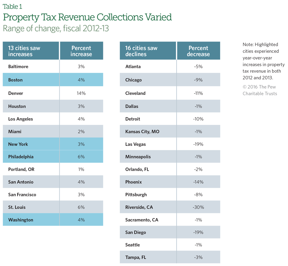
Thirteen of the cities recorded increases in property tax revenue over the previous year. Sixteen cities experienced year-over-year declines in property taxes in fiscal 2013, compared with 24 cities in 2012, and the losses on average were smaller. Still, many continued to deal with the effects of depressed property values long after the Great Recession’s end in July 2009. The cities that recorded drops in property tax collections did so in part because of the lag in assessment updates reflecting lower home values after the recession. (See Table 1.) The lag in property assessments also translated into slower improvement in property tax revenue once the real estate market started to climb again.
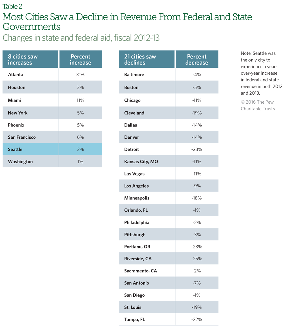
In fiscal 2013, state and federal aid, a critical revenue source for local governments, declined in 21 of the 29 cities. The reductions, at an average of 6 percent between fiscal 2012 and 2013, proved steeper than in any year since the Great Recession began. The cuts in state aid reflected the deterioration in states’ own revenue during the recession and the slower-than-usual recovery that followed. Cities, like states, must balance their budgets each year, so they have to offset revenue reductions from the state by some combination of cutting spending, increasing taxes and fees, dipping into reserves, selling assets, or borrowing short term.
On a more positive note, revenue from sales and personal income taxes rose in most cities in fiscal 2013 because of increases in consumer spending and slowly improving employment. Eighteen of the 20 cities with a sales tax saw year-over-year increases from fiscal 2012, representing the fourth straight year of sales tax growth, when looking at the average change, across these cities. Eight of the nine cities that collect local income taxes reported increases, representing the third straight year of income tax growth, on average, across these cities.
Spending trends
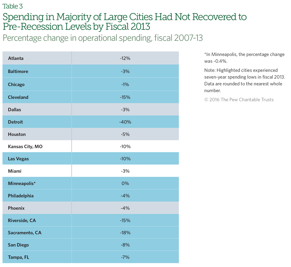
By fiscal 2013, operational spending still had not recovered to 2007 levels in a majority of the 29 cities. In fact, more than a third faced seven-year lows.
Confronting slow revenue growth, officials in cities across the country made strikingly different choices about where to reduce expenses. For example:
- 17 cut overall spending, with the most common reductions in two categories: debt and housing and economic development.
- Portland reduced overall spending by 13 percent after two consecutive years of growth. The city trimmed debt service expenditures in part by refinancing existing debt and chopped housing and economic development costs by 31 percent.
- Tampa cut spending for public safety by 13 percent, housing and economic development by 45 percent, and general government (which covers operational functions, such as the mayor’s office, and other functions within City Hall that fall outside other major service-delivery categories) by 28 percent in fiscal 2013.
- The cities that reduced year-over-year spending cut their expenditures by an average of 7 percent, the deepest average reductions in the seven years examined by Pew.
- Continued belt-tightening proved painful. In many cases, spending cuts were difficult because they followed several years of similar measures in response to sustained revenue declines. As a result, 11 cities reached seven-year operational spending lows in fiscal 2013.
- In a sign of the lingering impact of the recession, more than half of the cities reached spending lows for the years studied in 2012 or 2013, even as the nation’s economy was well into the recovery.
- Cleveland cut overall operational spending every year from 2008 to 2013. Over that period, expenditures fell from $804 million to $664 million, or 17 percent.
- In Sacramento, city officials sounded an alarm in their 2013 Comprehensive Annual Financial Report, warning, “Despite significant progress in realigning its revenues and expenditures, the City’s financial position is not secure and more difficult decisions will need to be made. … [W]e must continue to reevaluate not only how we deliver services and meet citizen needs, but also which programs and services the City can afford to deliver if expenditure growth continues to outpace that of revenue.”1
By fiscal 2013, operational spending still had not recovered to 2007 levels in a majority of the 29 cities. In fact, more than a third faced seven-year lows. Confronting slow revenue growth, officials in cities across the country made strikingly different choices about where to reduce expenses.
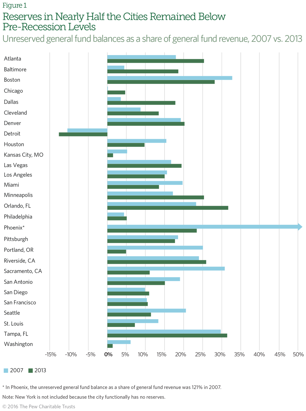
Update on reserve balances
Reserves are important fiscal management tools for governments of all sizes. They afford policymakers a fiscal cushion to close budget gaps, temporarily maintain city services, and mitigate the impact of falling revenue collections. After many cities dipped into their savings in the years following the Great Recession, cities generally showed larger balances in fiscal 2013, suggesting that some took advantage of moderate post-recession growth to start rebuilding their financial cushions. (A New York state mandate prohibits New York City from carrying reserve balances, so it is not included in the reserves analysis. For more information, see the full methodology.)
- Of the 23 cities that increased their general fund balances, the average balance-to-revenue ratio rose from 11 percent in 2012 to 14 percent in 2013.
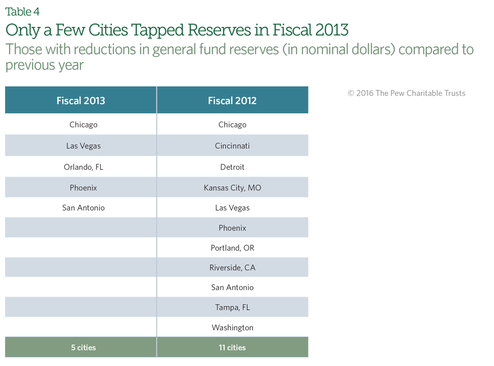
- Fewer cities tapped their reserve funds in 2013 compared with the previous year. In fiscal 2013 just five did so, compared with 11 in fiscal 2012. (See Table 4 for a list of cities that used reserves in each year.)
- Still, balance-to-revenue ratios in 14 cities remained below pre-recession levels. (See Figure 1.)
Municipal bond issuances
To understand borrowing activity in large cities, Pew also analyzed inflation-adjusted calendar year data from the Thomson Reuters SDC Platinum database covering municipal bond issuances over the last three recessions and the recovery periods that followed. Because it is based on a different data source, this analysis includes Cincinnati and brings the total to 30 cities. Among the key findings:
- In 2014, new money bond issuances in the 30 cities hit their lowest point in a 24-year period that started in 1991. This contradicted usual borrowing patterns following economic downturns. Sales of new money bonds typically rise during a recovery as interest rates are often low, but from 2010 through 2014 total new money issuances for these cities averaged only $12.2 billion annually.
- In 2014, the 30 cities analyzed issued $9.8 billion in new money bonds, compared with $12.4 billion in 2007 as the nation headed into the Great Recession. Not all of these cities issued new money bonds, but of those that did the amount sold varied widely, from $6.5 million in Tampa to $1.5 billion in Chicago.
- The refinancing of bonds, known as refunding, totaled $9.2 billion in 2014—nearly half (49 percent) of total bonds issued.2Since 2011, refunding has consistently exceeded 40 percent of bond issuances in the cities.
For the full analysis on municipal issuances, please see “Issuance of New Money Bonds Remains Low in Large U.S. Cities.”
Methodology and definitions
The following describes the methodological approach and terms used in The Pew Charitable Trusts’ issue brief “Fiscal Health of Large U.S. Cities Varied Long After Great Recession’s End.”
The analysis, based on audited city financial statements, continues work undertaken by Pew following the Great Recession, which ran from late 2007 through mid-2009. For this multiyear series, Pew has examined data in the financial statements of the central city in each of the nation’s 30 largest metro areas as defined by the 2010 census. Though included in previous analyses, Cincinnati was excluded from the most recent look at revenue, spending, and reserves because city officials changed its fiscal year in 2013. That resulted in financial documents that covered only six months and made it impossible to compare financial information to previous years or to other cities included in the analysis.3
A separate brief, “Issuance of New Money Bonds Remains Low in Large U.S. Cities,” looks at trends in city bond issuances through 2014 and uses a different set of data, so the methodology is different as well.
Data and methods
The primary data sources for this analysis are Comprehensive Annual Financial Reports (CAFRs) for fiscal 2007 through 2013. Pew researchers collected data from the statement of revenues and expenditures and the statistical section of each city’s CAFR for every year in the study period.4 This analysis considers all governmental revenue and expenditures and is not limited to those just from each city’s general fund.5Although each city is unique, Pew organized governmental revenue and expenditure line items into major groupings that are comparable across cities. A detailed description of these groupings is given in the revenue and expenditures sections of this document.
Controlling for the effects of inflation enables comparisons of how fiscal conditions have changed for cities over the period studied and in relation to each other. Dollars are adjusted for inflation using the U.S. Bureau of Economic Analysis’ National Income and Product Account estimate. The same gross domestic product deflator values were used for all 29 cities in the 2013 analysis, regardless of geographic location, though each was adjusted to accommodate the appropriate fiscal year calendar in a given city. This approach avoids overstating differences between cities based solely on imperfect inflation estimates.6
Data limitations
There are several differences inherent to the governments of the 29 cities that data adjustments cannot standardize, such as the services they provide, the ways they generate revenue, their governmental structures, and their relationships with surrounding local and state governments. Although we have standardized the data across cities to the greatest extent possible and have consulted with the cities and adjusted data where appropriate, readers should keep these differences in mind.
In a few cases, variations from the standard methodology were required because of data constraints. Philadelphia, St. Louis, and Seattle, for example, did not break out revenue categories consistent with the detail provided by the other cities. After consulting with these cities, researchers relied on data from the supplemental statistical section of the CAFR (for Seattle and St. Louis) and detailed, supplemental financial reports (for Philadelphia). The modifications result in minor differences between the values of the line items used in this research and the values reported in the CAFR’s statement of revenues and expenditures.7
The remittance of the city share of state-imposed taxes, specifically sales tax, utility tax, and communication service tax in Florida, is reported differently in city CAFRs, especially as it affects Miami and Tampa, Florida. In some instances, these taxes are reported as own-source revenue, though they are locally generated state revenue that the city receives from the state. Pew re-categorized and included this revenue as intergovernmental to ensure accurate cross-city comparisons.
Analytical approach
Pew researchers identified a “peak” and “trough” revenue year for each city, using inflation-adjusted dollars. Peak years could occur at any point in the study period, while trough years were defined as the lowest revenue point between 2008 and 2013; this time frame specifically targets revenue declines generated by the Great Recession.8Next, Pew grouped cities based on 2013 revenue performance relative to each city’s prior peak to identify those experiencing a rebound—exceeding their previous revenue high points—and those still struggling to return to pre-downturn levels.
For each city, Pew examined the primary drivers of revenue loss between peak and trough years, calculated the total revenue decline, and analyzed the share of that total loss represented by each individual revenue source. Similarly, for rebounding cities, Pew identified the revenue streams that were most responsible for financial gains between a city’s trough year and the end of the study period, as well as between 2012 and 2013. This strategy allowed researchers to assess trends across cities in the types of losses that drove revenue declines and the gains that spurred rebounds.
Revenue
Pew researchers normalized revenue data reported in city CAFRs to create comparable categories that allow for meaningful comparisons across cities. While some types of revenue are reported relatively consistently across cities, in other cases Pew combined CAFR line items to create similar revenue groupings across cities. The categories include:
- Property tax. All revenue that is raised through taxes on the value of property, including residential, commercial, industrial, and other types of property.
- Sales tax. All revenue that is raised through the direct imposition of local option sales taxes by a city.9
- Income tax. All revenue that is raised through a city’s direct imposition of personal income and wage taxes.10
- Other tax revenue. All tax revenue raised through a city’s direct imposition besides property taxes, sales taxes, and income taxes. For many cities, this category includes special local taxes on hotels, utilities, gasoline, occupancy, alcohol, and/or gross business receipts.
- Intergovernmental revenue. All grants, transfers, and other funding streams that the city receives from other governments at all levels, including federal, state, and local. Because only a handful of cities list intergovernmental aid by source in their CAFR, it is not possible to separate federal, state, and local aid.
- Charges and fees. All funding that cities collect through the imposition of licensing and user fees, such as vehicle registration fees, traffic tickets, construction permits, fines and forfeitures, and payments in lieu of taxes.
- Other nontax revenue. All remaining types of revenue that are not captured in the other categories and that are not collected as taxes, such as donations to government by individuals, income (or loss) from investment decisions, income from the sale and leasing of city capital assets, and income from the rental of city-owned buildings.
Expenditures
Pew researchers also examined how cities responded to revenue decline and growth by looking at changes in operating spending, reserves, and the management of long-term obligations.11Applying the same approach as with city revenue, researchers grouped CAFR line items where appropriate to create comparable spending categories across the cities. The categories include:
- Public safety. Expenditures on police, fire, emergency, and judicial services.
- Social and health services. Expenditures on hospitals, mental health, Medicaid, welfare, and public health.
- Housing and development. Expenditures on housing and economic development activities.
- Public works and transportation. Expenditures on existing infrastructure, utilities (including water and sewer/ sanitation), roads, and public transportation provision and maintenance.12
- Parks, recreation, and cultural facilities. Expenditures on public parks and recreational and cultural facilities, including city-run museums, libraries, and convention centers.
- Education. Expenditures on K-12 education. While schools in 25 of the cities studied are run by separate school boards and authorities, four cities directly provide education.
- General government. Expenditures on operational functions, such as the mayor’s office, and other functions within City Hall that fall outside other major service-delivery categories.
- Debt service. Expenditures on debt including interest, principal payments, and bond issuance costs.
- Other. All spending that does not fit into another category. It can include such things as retirement benefits (if they are not part of a separate pension fund), other employee benefits (if they are not included in the departments where the employees work), and claims and judgments.
Reserves
Pew measured each city’s available general fund balance as a percentage of total general fund revenue to account for its capacity to fund operations in the face of large and/or sustained budget shortfalls. Pew’s assessment of reserves was limited to the available general fund balance (as opposed to assessing balances across total governmental funds) in an effort to create a standardized measure across the cities.13
Endnotes
- City of Sacramento, Comprehensive Annual Financial Report for Fiscal Year 2013, p. iii.http://portal.cityofsacramento.org/Finance/Accounting/Reporting.
- Because of incomplete data reporting by the cities, some bonds reported in the Thomson Reuters SDC Platinum database as new money were in fact used for refunding purposes. Due to these errors, the amount of new money bonds could be lower than reported here, and the amount of refunding bonds higher.
- The cities studied in the brief “Fiscal Health of Large U.S. Cities Varied Long After Great Recession’s End” are Atlanta; Baltimore; Boston; Chicago; Cleveland; Dallas; Denver; Detroit; Houston; Kansas City, Missouri; Las Vegas; Los Angeles; Miami; Minneapolis; New York; Orlando, Florida; Philadelphia; Phoenix; Pittsburgh; Portland, Oregon; Riverside, California; Sacramento, California; San Antonio; San Diego; San Francisco; Seattle; St. Louis; Tampa, Florida; and Washington.
- Mandated by state law, Comprehensive Annual Financial Reports (CAFRs) are final, audited statements of city revenue, expenditures, reserves, and debt. CAFR data were chosen for two reasons. First, CAFRs present city fiscal data that have been reviewed by an outside auditor and are considered final. Other financial documents, such as budgets, are more fluid and tend to be subject to revisions throughout the year as city priorities change. Second, data in CAFRs are standardized by the Governmental Accounting Standards Board 11 (GASB) and must comply with Generally Accepted Accounting Principles. Although there are some differences in the way CAFR data are presented from city to city, these documents are much more standardized than other city financial documents.
- The fiscal organization of large cities varies widely. For example, in Phoenix the general fund accounts for about 14 percent of total governmental revenue, while in New York the general fund represents almost 94 percent. Among the 29 cities in this analysis, the general fund typically accounts for about two-thirds of total governmental revenue, which means about one-third of fiscal activity is missed if the general fund is the singular focus of the analysis. This analysis excludes proprietary or enterprise funds generated by the city for specific purposes such as the operation of programs or agencies that are self-sustaining or revenue-positive.
- Inflation adjustments using National Income and Product Account estimates better reflect the inflation pressures facing local governments (as compared with, for example, the consumer price index) but are not a perfect measure of the “basket of goods” for which government entities are responsible. Although this analysis strives to correct for year-over-year changes in the value of the dollar, it is important to not overstate differences between city fiscal conditions based only on the value of a deflator.
- Because Philadelphia has a unique relationship with the state of Pennsylvania resulting from the ongoing existence of the Pennsylvania Intergovernmental Cooperation Authority (PICA)— formed to stabilize the city’s finances—Philadelphia’s CAFR document does not present line items for revenue either in the statement of revenues and expenditures or in the statistical section. Note that Pittsburgh also has an ongoing relationship with PICA, but it does not affect the way it presents information in its CAFR.
- Including 2007 as a “low” will, for some cities with strong revenue performance, simply capture the earliest point in time, not the impact of the Great Recession on revenue.
- This category does not include sales tax revenue that states or counties impose and collect, and then remit a portion of to the cities—that is captured in intergovernmental aid.
- Income taxes imposed and collected by the state and/or county from which a portion is remitted to cities are captured in intergovernmental aid.
- Operating spending is defined as total governmental expenditures less capital outlays. Three cities—Atlanta, New York, and Pittsburgh— do not separate out capital outlays spending as a line item in their CAFR document, instead reporting capital spending by department in a capital projects fund. Atlanta and New York have done this throughout each year of the six years of analysis, while Pittsburgh began using this method in 2012. In these three cases, Pew consulted with city officials to arrive at estimates of total capital spending and to reduce expenditure line items appropriately.
- In San Antonio, spending categorized as “sanitation” in the city’s CAFR is dedicated to food inspections. As such, we have included these expenditures under the social services/health category in order to facilitate accurate cross-city comparisons. Note that for all cities, expenditures to expand infrastructure, utilities, roads, and public transportation are accounted for in capital outlays.
- Financial reporting requirements that govern the CAFR result in standardized reporting across the cities’ general fund reserves; this is not the case for balances across other funds. However, note that over the period the report examines, some cities became early adopters of GASB rule No. 54, which changes the way cities report year-end fund balances from two categories (reserved and unreserved) to four (restricted, committed, assigned, and unassigned). See Governmental Accounting Standards Board, “Summary of Statement No. 54” (February 2009),http://www.gasb.org/st/summary/gstsm54.html. For these cities, only the money reported as assigned and unassigned was included as unreserved general fund balances. This treatment is the most consistent with the previous definition and with how cities made the transition in reporting.


ADDITIONAL RESOURCES

Article


